Contents
Parallel Implementation Design
The parallel application of simulating Rayleigh–Bénard convection in a two-dimensional grid is tightly-coupled and compute-intensive (HPC) in which independent parallel tasks are performed simultaneously.
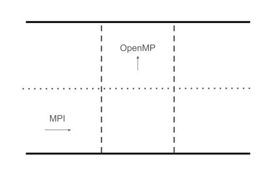
We use a pencil domain decomposition in the horizontal direction, to distribute the temperature, velocity fields, Fourier modes and other relevant arrays across processors using MPI. Employing the FFTW MPI library we allocate local arrays to each processor and use task level parallelism to perform parallel 1D FFT transforms. We also make use of shared-memory processing (i.e. procedure level parallelism) by employing OpenMP to parallelize loops in the vertical direction.
Initialization of the fields is performed locally on each node and we use distributed I/O to export local field arrays during the simulation. A separate utility function is used to combine the output from the individual processes into a single file representing the entire domain.
The distributed-memory, multi-node implementation enables us to scale to much larger problems, given that the problem size is not constrained by the memory of a single node.
We manage to achieve a material speed up in execution time as we increase the number of processors for a sufficiently large problem. Detailed analysis is included in the Benchmarking section.
Overview of Serial Code
The original serial code algorithm is used to find steady solutions to the 2D Boussinesq equations. The envisaged use-case for the parallel version of the code is mainly to serve as a time integrator, used to evolve the temperature and velocity fields over time for a given set of initial conditions - i.e. not explicitly solving the steady state solution. Based on the performance analysis of the serial code the time integrator is also the most compute intensive component of the process. As such we remove the flowmap components from the original code and focus on the time integrator module.
We present a brief overview of the main scripts included in the serial version of the code to provide additional context for the subsequent sections in the report:
allocate_vars.f90: Arrays allocated and initializedbc_setup.f90: Boundary conditions setupfftw_mpi.f90: FFTW module importedglobal.f90: Global variablesmesh_pack.f90: Cosine mesh initializedstatistics.f90: Utility functionstime_integrators.f90: Time integratorTime_loop.f90: Main program (imports data and runs time integrator)
FFTW MPI
Background
FFTW is a widely used free-software library that computes the discrete Fourier transform (DFT) and its various special cases. Its performance is competitive even with vendor-optimized programs:
- Written in portable C and runs well on many architectures and operating systems
- Adapts to specific hardware architecture
- Computes DFTs in $O(n log n)$ time for any length $n$
- Includes a Fortran wrapper
Fortran 2003 standardized ways for Fortran code to call C libraries, and this allows FFTW to support a direct translation of the FFTW C API into Fortran, which we employed in this project. Some important things that we had to consider when we implemented the code includes:
- The MPI routines are significantly different from the serial FFTW routines because the transform data here are distributed over multiple processes, so that each process gets only a portion of the array
- Functions in C become functions in Fortran if they have a return value, and subroutines in Fortran otherwise
- The ordering of the Fortran array dimensions must be reversed when they are passed to the FFTW plan creation, thanks to differences in array indexing conventions
- Special C data types had to be used for the FFTW plans and allocated arrays and pointers
Implementation
The serial code base uses the FFTW library to transform variables between physical and Fourier space at different points in the process, with several transforms being performed at each time step.
A significant part of the project involved us developing a firm understanding of the FFTW MPI API and replacing the serial FFTW functions with the parallel functions. Special care was taken to ensure that the functions provided the expected output.
At a high level the FFTW MPI implementation consists of the following steps:
- Determine local array sizes based on size of horizontal domain ($N_x$) and number of processors specified by MPI run (nproc)
- Allocate double complex array pointers on local nodes for each of the relevant fields
- Perform C to Fortran pointer conversion
- Create forward and backward FFT plans for each of the fields
- Run FFT transforms as required
We note that communication between tasks is effectively limited to the FFT transforms, but that a large number of these executions are performed at each step in the time integrator. It can therefore still present a significant communication bottleneck, which we evaluate in the Benchmarking section.
The FFTW MPI implementation is primarily contained in the following scripts:
global.f90time_integrators.f90Time_loop.f90
OpenMP
Using OpenMP we parallelize loops in the vertical direction ($N_y$) using multi-processing. Recall that FFTW MPI is used to distribute data in the horizontal direction. Given that a separate 1D FFT call is required for each element for each horizontal slice in $N_y$, using multiple threads should increase the parallel performance of the code.
!$OMP PARALLEL DO
do j = 1,Ny
! Bring everything to physical space
tnlT   = nlT(j,:)
tnlphi = nlphi(j,:)
tT     = Ti(j,:)
tux    = uxi(j,:)
tuy    = uyi(j,:)
tphi   = phii(j,:)

call fftw_mpi_execute_dft(iplannlT, tnlT, tnlT)
call fftw_mpi_execute_dft(iplannlphi, tnlphi, tnlphi)
call fftw_mpi_execute_dft(iplanT, tT, tT)
call fftw_mpi_execute_dft(iplanux, tux, tux)
call fftw_mpi_execute_dft(iplanphi, tphi, tphi)
call fftw_mpi_execute_dft(iplanuy, tuy, tuy)

nlT(j,:)   = tnlT
nlphi(j,:) = tnlphi
Ti(j,:)   = tT
uxi(j,:)  = tux
uyi(j,:)  = tuy
phii(j,:) = tphi

end do
!$OMP END PARALLEL DO
Parallel I/O
Given that the domain is now distributed across multiple nodes, the I/O used in serial code needs to be adapted. In order to minimize communication between tasks, each node exports the relevant solutions to disk. A separate Python utility function is developed to import and combine the solutions into the complete domain.
The input file (see Reproducibility section) allows the user to specify what output should be produced. The main outputs produced by the process are:
- VTK data files: Structured text output of grid and temperature and velocity fields exported at the end of the simulation
- Field solution: Text files with raw data temperature ($T$) and velocity fields ($u_y$) at fixed time intervals
- Nusselt number at fixed intervals
Given the importance of the Nusselt number ($Nu$) as a diagnostic quantity, we compute the value at fixed intervals in the time integrator (the interval length is a parameter of the imex_rk function called in the Time_loop.f90 script). In order to compute the Nusselt value for the entire solution, it is first calculated locally by each node and then aggregated using an all-to-all MPI Gather communication.
Advanced Features
The main challenge of this project was to integrate all the different components of the parallel design within a complex code base. We had very limited familiarity with the different applications used in the project and had to quickly develop a working knowledge of Fortran, FFTW and MPI as well as an adequate understanding of the underlying mathematics used in the code. We found the limited online documentation available for debugging issues related to Fortran and the 1D FFTW implementation in particular quite challenging.
What also made this project unique was the understanding that the parallel code could likely be used for future research. As such we devoted significant time to validate the output from the parallel code by reconciling it to the serial code output. During this process, we also identified a minor allocation problem within the serial code, that we successfully resolved. We successfully reconciled results to machine-level accuracy.
Sample Output
As noted above the main output produced by the code is the temperature and velocity field solutions at different timesteps. Below we include simulated output produced using the parallel code.
$Ra$ = 50,000 and 1000 time steps
$Ra$ = 500,000 and 10,000 time steps

Validation of Parallel Code
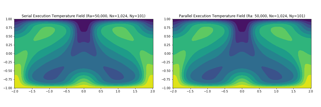
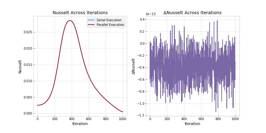
In this section we include some of the analysis we performed in order to validate the output of the parallel code (and thereby ensure consistency with the serial code). To this extent, the Temperature Fields were compared after a given number of iterations whereas Nusselt Numbers were compared at every iteration.
We began by running the serial code with Ra=5000 and Nx=128 and outputting the Temperature Field after 100 iterations as well as outputting the Nusselt Number at every iteration. We then ran the MPI only version with Nproc = 1,2,4 and 8 (limited to 8 when Nx =128) and also ran the MPI/OpenMP hybrid parallel version with the same number of Nprocs and varied OMP_NUM_THREADS as well as -c flags.
To compare the fields we used the infinity norm of the difference between the parallel and serial versions. Our results showed that all the configurations (both MPI and MPI/OpenMP) produce an infinity norm of 1E-11 or lower. Furthermore, we ran the same experiment with Ra=50,000 and Nx = 1024 and again validated the output of the parallel code.
As a final validation we compared parallel versions which ran on N > 1 (number of nodes) and obtained the same results as we did using a single node, validating the distributed-memory component of the code. Given these results, we are confident that the parallel implementation is consistent with the serial code base.
Results from one of the runs are highlighted in the figure below as well as a table containing results from all the runs:
Ra = 5000, nx = 128, ny = 101
MPI Only
| Field | MPI (1 proc) | MPI (2 proc) | MPI (4 proc) | MPI (8 proc) |
|---|---|---|---|---|
| T | 2.49E-12 | 7.55E-12 | 3.67E-12 | 4.64E-12 |
| Nu | 2.47E-12 | 2.61E-12 | 2.46E-12 | 2.10E-12 |
MPI/OpenMP Hybrid
| Field | MPI+OMP (1 proc) | MPI+OMP (2 proc) | MPI+OMP (4 proc) | MPI+OMP (8 proc) |
|---|---|---|---|---|
| T | 6.73E-12 | 7.55E-12 | 3.67E-12 | 4.64E-12 |
| Nu | 2.47E-12 | 2.61E-12 | 2.46E-12 | 2.10E-12 |
Ra = 50,000, nx = 1,024, ny = 101
MPI Only
| Field | MPI (1 proc) | MPI (2 proc) | MPI (4 proc) | MPI (8 proc) |
|---|---|---|---|---|
| T | 2.18E-11 | 1.81E-11 | 2.97E-11 | 3.94E-11 |
| Nu | 1.14E-13 | 1.16E-13 | 1.19E-13 | 1.33E-13 |
MPI/OpenMP Hybrid
| Field | MPI+OMP (1 proc) | MPI+OMP (2 proc) | MPI+OMP (4 proc) | MPI+OMP (8 proc) |
|---|---|---|---|---|
| T | 2.18E-11 | 1.81E-11 | 2.97E-11 | 3.94E-11 |
| Nu | 1.14E-13 | 1.16E-13 | 1.19E-13 | 1.33E-13 |
References
Frigo, M. and Johnson, S.G., 2005. The design and implementation of FFTW3. Proceedings of the IEEE, 93(2), pp.216-231
Poel, Erwin P van der, et al. 2015. “A pencil distributed finite difference code for strongly turbulent wall- bounded flows”. Computers & Fluids 116:10–16